Rock-Paper-Scissors

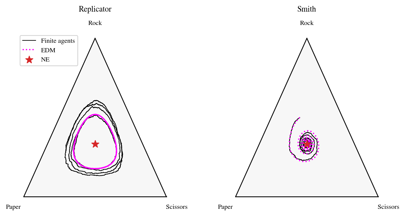
This example models a population of agents playing the classic Rock-Paper-Scissors game, where each strategy beats one strategy and loses to the other. The unique Nash equilibrium (NE) is the uniform distribution \((1/3, 1/3, 1/3)\).

It compares two revision protocols and shows how they can lead to very different long-run behavior, even when the game has the same equilibrium:

• Replicator (pairwise proportional imitation): agents imitate better-performing opponents. The resulting evolutionary dynamics model (EDM) is the replicator dynamics, whose trajectories are closed orbits around the NE (the product \(x_1 x_2 x_3\) is conserved). With finitely many agents, random fluctuations make the population drift across orbits.

• Smith: agents switch to strategies with higher payoff than their current one, regardless of how popular they are. The population converges to the NE.

import numpy as np
import matplotlib.pyplot as plt
import ternary
from popgames import (
    SinglePopulationGame,
    PayoffMechanism,
    PoissonRevisionProcess,
    Simulator,
)
from popgames.revision_protocol import Replicator, Smith

A = np.array([[0, -1, 1],    # Rock
              [1, 0, -1],    # Paper
              [-1, 1, 0]],   # Scissors
             dtype=float)    # floats, so that the example also runs with the numba backend

def fitness_function(x):
    return np.dot(A, x)

population_game = SinglePopulationGame(
    num_strategies=3,
    fitness_function=fitness_function,
)

payoff_mechanism = PayoffMechanism(
    h_map=fitness_function,
    n=3,
)

revision_protocols = {
    'Replicator': Replicator(scale=0.5),
    'Smith': Smith(scale=0.25),
}

x0 = np.array([0.5, 0.3, 0.2]).reshape(3, 1)
T_sim = 100

fig, axes = plt.subplots(1, 2, figsize=(8, 4))

for ax, (name, revision_protocol) in zip(axes, revision_protocols.items()):
    revision_process = PoissonRevisionProcess(
        Poisson_clock_rate=1,
        revision_protocol=revision_protocol,
    )

    sim = Simulator(
        population_game=population_game,
        payoff_mechanism=payoff_mechanism,
        revision_processes=revision_process,
        num_agents=1000
    )

    sim.reset(x0=x0)
    out = sim.run(T_sim=T_sim)
    edm = sim.integrate_edm_pdm(t_span=(0, T_sim), x0=x0, t_eval=np.linspace(0, T_sim, 2000))

    _, tax = ternary.figure(ax=ax, scale=1)
    tax.boundary(linewidth=1.0)
    tax.plot(out.x[[2, 0, 1], :].T, linewidth=0.8, color='black', label='Finite agents')
    tax.plot(edm.x[[2, 0, 1], :].T, linewidth=1.5, linestyle='dotted', color='magenta', label='EDM')
    tax.scatter([(1/3, 1/3, 1/3)], marker='*', s=80, color='tab:red', zorder=3, label='NE')
    tax.top_corner_label('Rock')
    tax.left_corner_label('Paper')
    tax.right_corner_label('Scissors')
    tax.clear_matplotlib_ticks()
    tax.get_axes().axis('off')
    tax.set_title(name, pad=25)

axes[0].legend(loc='upper left', fontsize=8)
plt.subplots_adjust(wspace=0.35)
plt.show()

Running with the Numba backend

Both simulations can run with the optional Numba backend (requires pip install "popgames[numba]") by adding backend="numba" to the simulator:

sim = Simulator(
    population_game=population_game,
    payoff_mechanism=payoff_mechanism,
    revision_processes=revision_process,
    num_agents=1000,
    backend="numba",
)

The payoff matrix is declared with dtype=float. The fitness function is compiled automatically with numba.njit, and Numba does not support matrix products between integer and floating-point arrays: with an integer matrix such as np.array([[0, -1, 1], [1, 0, -1], [-1, 1, 0]]), compilation fails, and the simulator logs a warning and falls back to the numpy backend. Writing the entries as floats (e.g., 0.0) works as well.

If you prefer to compile the fitness function explicitly, decorate it with @numba.njit:

import numba

@numba.njit
def fitness_function(x):
    return np.dot(A, x)

Both simulators use the same fitness function, which is therefore compiled only once. Both revision protocols are built-in, so they are supported by the Numba backend.

With 1000 agents over 100 time units (about 100 000 revision events per protocol), the compilation time is comparable to the time saved, so both backends take about the same time. For larger populations, e.g., num_agents=100_000, the Numba backend is about 100 times faster than the numpy backend.