Getting Started
PopGames is a Python library for modeling and simulating population games.
Source Code
🔗 GitHub repository:
https://github.com/Martinez-Piazuelo/popgames
Installation
PopGames is available on PyPI and can be installed using pip.
Install from PyPI
pip install popgames
This installs the latest released version together with its dependencies.
Install the development version
If you want the latest features, you can install the development version directly from GitHub:
pip install git+https://github.com/Martinez-Piazuelo/popgames.git
Optional: Numba backend
To speed up large simulations with the optional Numba backend, install the
numba extra:
pip install "popgames[numba]"
Numba is only needed when a simulator is created with backend="numba".
Verify the installation
You can verify that PopGames is installed correctly by running:
import popgames
print(popgames.__version__)
If no errors occur, the installation was successful.
Quick Usage Example
PopGames follows an object-oriented design built around four core components:
Population game: defines the strategic environment
Payoff mechanism: specifies the payoff perceived by agents
Revision process: determines how agents update their strategies
Simulator: orchestrates and runs the simulation
This example demonstrates how to simulate a simple population game using popgames.
We model the classic Prisoner’s Dilemma, where agents repeatedly choose between two strategies:
Cooperate
Defect
Although mutual cooperation is socially optimal, evolutionary dynamics often drive the population toward defection.
Define the fitness function
We begin by defining the fitness function for the Prisoner’s Dilemma. The payoff parameters satisfy
T > R > P > S
where:
T – temptation to defect
R – reward for mutual cooperation
P – punishment for mutual defection
S – sucker’s payoff
The fitness function is then of the form:
f(x) = [[R, S], [T, P]]x
which can be implemented in Python as follows:
import numpy as np

T, R, P, S = 3, 2, 1, 0

def fitness_function(x):
    return np.dot(
        np.array([[R, S], [T, P]]),
        x
    )
Create the population game and payoff mechanism objects
Next we instantiate the population game and payoff mechanism objects by specifying the number of strategies and the fitness function.
from popgames import (
    SinglePopulationGame,
    PayoffMechanism,
)

population_game = SinglePopulationGame(
    num_strategies=2,
    fitness_function=fitness_function,
)

payoff_mechanism = PayoffMechanism(
    h_map=fitness_function,
    n=2,
)
Define the revision process object
Agents revise their strategies according to a Poisson revision process combined with a softmax revision protocol. We therefore define the corresponding revision process object as follows.
from popgames import PoissonRevisionProcess
from popgames.revision_protocol import Softmax

revision_process = PoissonRevisionProcess(
    Poisson_clock_rate=1,
    revision_protocol=Softmax(0.1),
)
Instantiate the simulator and run the simulation
We now create the simulator and run the population dynamics. The simulation considers a population of 1000 agents starting from an equal split between the two strategies.
from popgames import Simulator

sim = Simulator(
    population_game=population_game,
    payoff_mechanism=payoff_mechanism,
    revision_processes=revision_process,
    num_agents=1000
)

x0 = np.array([0.5, 0.5]).reshape(2, 1)  # Initial state

sim.reset(x0=x0)
out = sim.run(T_sim=30)
Visualize the results
Finally, we visualize the evolution of the population state using matplotlib.
import matplotlib.pyplot as plt

plt.figure(figsize=(3, 3))

plt.plot(out.t, out.x[0, :], label="Cooperators")
plt.plot(out.t, out.x[1, :], label="Defectors")

plt.xlabel("Time")
plt.ylabel("Population fraction")
plt.legend()
plt.grid()

plt.tight_layout()
plt.show()
PopGames also provides built-in visualization utilities supporting ternary plots, univariate projections, and custom key performance indicators. For more details, see the API reference documentation.
Run an ensemble of simulations
Finite-agent simulations are stochastic, so a single run shows only one possible outcome.
run_ensemble runs many simulations and samples them at common times, either from the same initial state with
different seeds, or from different initial states:
# Same initial state, 20 different seeds
ens = sim.run_ensemble(T_sim=10, num_runs=20, x0=x0, seed=0)
ens.plot(plot_type="bands", variables=["x"], plot_deterministic_approximation=True)

# 10 random initial states, same seed
from popgames.utilities import sample_initial_states

x0s = sample_initial_states(population_game, num=10, seed=1)
ens = sim.run_ensemble(T_sim=10, x0=x0s, seed=[0] * len(x0s))
ens.plot(plot_type="kpi", plot_deterministic_approximation=True)
The result holds the runs in arrays of shape (runs, strategies, times) (e.g., ens.x), with helpers such as
ens.mean() and ens.quantile(...), and plots of quantile bands, KPIs, ternary trajectories, and final states.
See the usage examples in the documentation for more details.
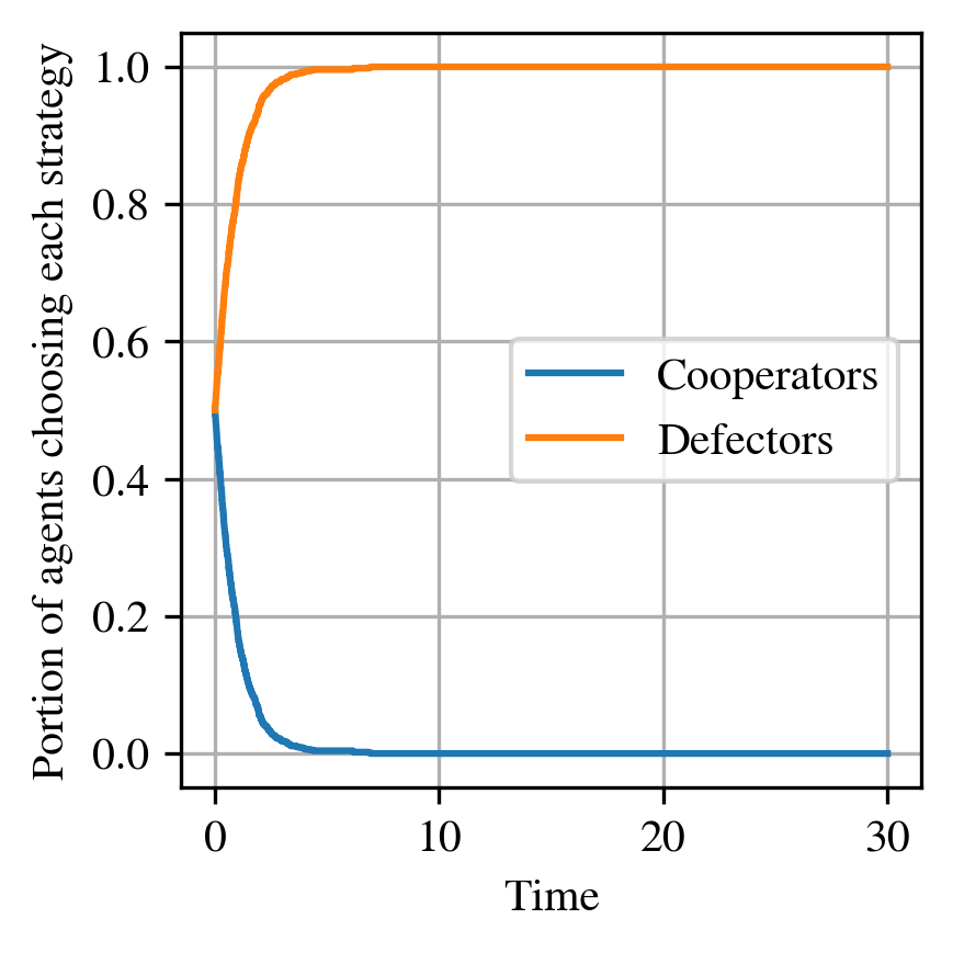
For the considered example, if everything works as expected, you should see a plot like:
What happens?
Starting from a balanced population, the evolutionary dynamics gradually favor defection, illustrating the well-known outcome of the Prisoner’s Dilemma in evolutionary settings.
Documentation
Usage Examples – hands-on full usage examples
Performance – faster simulations and the optional Numba backend
Key Concepts – connections with theoretical background
API Reference – full codebase documentation
Contributing to PopGames - how to contribute to the PopGames package